5 Qualitative Comparative Analysis (QCA) - operational procedure
5.1 Calibration
At this point, we have all the useful information to set the calibration. Our calibration will follow 2 axes: 1. calibration using statistics as categories cutting points; 2. calibration using natural gaps as cutting points.
Subsequently, for the ESG Overall Score we will have:
1. calibration using statistics have:
- exclusion point (e): Q20;
- cross over (c): Q50;
- inclusion point (i): Q80.
5.1.0.1 Function Set up - seeGaps & descriptive
The first step in the QCA Setup is to define the visualization function that graphically guide calibration decisions when empirical theories are unavailable.
seeGaps <- function(ID, X) {
  mydf <- cbind.data.frame(ID, X)
  mydf$X <- as.numeric(mydf$X)
  mydf$QQX <- as.factor(ntile(mydf$X, 10))
  ggdotchart(mydf, "ID", "X", color = "QQX",
             palette = c("#67001F","#B2182B", "#D6604D", "#F4A582",
                         "#FDDBC7","#D1E5F0", "#92c5DE", "#4393C3",
                         "#2166AC", "#053061"),
             sorting = "descending", add = "none", rotate = TRUE) +
    theme_minimal() +
    rremove("y.text") +
    geom_hline(yintercept = median(X), linetype = 3)
}
Similarly useful in terms of guiding us through calibration choices, is the function “descriptives” that gives us a sense of the main characteristics of the variables we will need to calibrate. It turns back information on the quantiles, in particular, the five quintile values, the minimum and maximum value of the variable, the mean and standard deviation.
descriptives <- function(x) {
  t <- data.frame(Min = min(x),
                  Q20 = quantile(x, 0.20),
                  Q25 = quantile(x, 0.25),
                  Mea = mean(x),
                  StD = sd(x),
                  Med = median(x),
                  Q75 = quantile(x, 0.75),
                  Q80 = quantile(x, 0.80),
                  Max = max(x)
  )
  t <- round(t, digits = 3)
  print(t, row.names = F)
}
5.1.1 ESG Overall Score - Calibration
To calibrate the ESG Overall Score, we start by putting the variable in question (OVERALL_SCORE) in a vector so that we can study it more straightforwardly.
C_OVERALL<- data$OVERALL_SCOREAt this point, we can produce a graph trough the seeGaps function and have the visualization of the silhouette of the data distribution. [Figure 2.1]
seeGaps(id, C_OVERALL)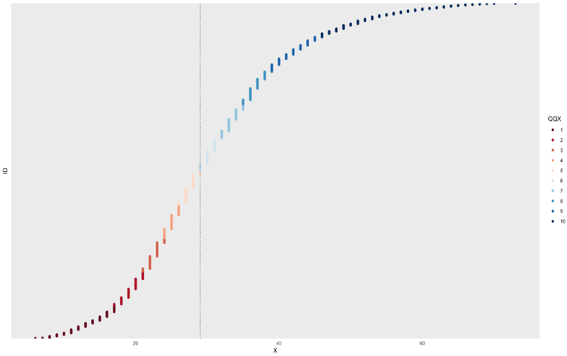 Figure 03.1
It can bee seen that the distribution is more compact for lower ESG Overall Scores and gets more rarefied through the right end of the graph.
Through the descriptives function, we get a sense of the variable distribution in a clear and quantitative way that will be helpful for the calibration choices that will be subsequently taken.
descriptives(C_OVERALL)| Min | Q20 | Q25 | Mea | StD | Med | Q75 | Q80 | Max |
|---|---|---|---|---|---|---|---|---|
| 6 | 21 | 23 | 30.394 | 11.271 | 29 | 37 | 39 | 73 |
Through the findTh function we get the natural gaps found in the distribution.
findTh(C_OVERALL, n= 1, method = "complete")By setting it at n=1, we get the first natural gap that results in 37.5. It is extremely near the Q75 value (37) meaning that the distribution is more compact below that point and less compact above it. This confirms the impression drawn from the seeGaps graphical visualization.
Setting the n=1 findTh is not enough to help with the calibration choices, for this reason we decide to set n to 7.
findTh(C_OVERALL, n= 7, method = "complete")This operation gives us the first 7 natural gaps that are:
| NatGaps | NatGaps | NatGaps | NatGaps | NatGaps | NatGaps | NatGaps |
|---|---|---|---|---|---|---|
| 13.5 | 21.5 | 29.5 | 37.5 | 53.5 | 65.5 | 37 |
At this point, we have all the useful information to set both the calibrations:
1. calibration using statistics as categories cutting points;
2. calibration using natural gaps as cutting points.
Subsequently, for the ESG Overall Score we will have:
1. calibration using statistics:
- exclusion point (e -> Q20): 21;
- cross over (c -> Q50): 30.394 ;
- inclusion point (i -> Q80): 39.
data$F_OVERALL_STAT<- calibrate(data$OVERALL_SCORE, type = "fuzzy", method = "direct",
                         thresholds = "e=21, c=30.394, i=39",
logistic = TRUE, idm = 0.953, ecdf = FALSE)- calibration using natural gaps:
- exclusion point (e -> forth natural gap, middle one): 29.5;
- cross over (c -> the first natural gap at the left of the middle gap): 37.5;
- inclusion point (i -> the first natural gap at the right of the middle gap): 45.5.
data$F_OVERALL_NATGAP<- calibrate(data$OVERALL_SCORE, type = "fuzzy", method = "direct",
                           thresholds = "e=29.5, c=37.5, i=45.5",
                           logistic = TRUE, idm = 0.953, ecdf = FALSE)
Both calibrations are then added to the data-set data.
5.1.2 2019 Revenues (log) - Calibration
As previously explained, the variable containing information for 2019 revenues has been transformed into logarithm to rescale the observations order of magnitude to compare different revenue values from case to case.
We put the variable for 2019 Revenues (LOG_REV_19) into a vector to lighten up the calibration analysis.
CALIB_LOGREV19 <- data$LOG_REV_19And subsequently proceed with the graphical representation of the variable trough the seeGaps function. [Figure 2.2]
seeGaps(id, CALIB_LOGREV19)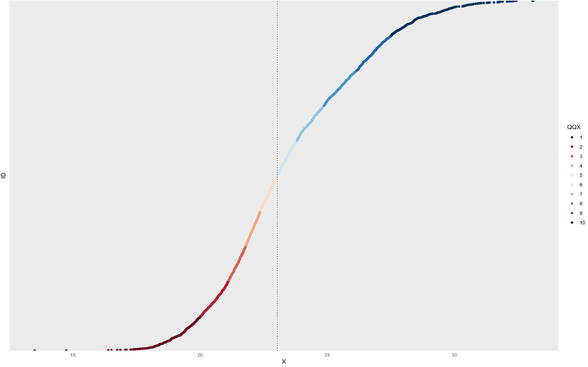
Figure 03.2
Since the original data-set did not come with any metadata specification, we are not sure whether the data for revenues comes as already fitted. The graph surely suggests it since it presents a regular smooth shape but we have no information on how the hypothetical fitting has been carried out.
Through the descriptives function, we get the quantitative crucial info of the variable distribution.
descriptives(CALIB_LOGREV19)| Min | Q20 | Q25 | Mea | StD | Med | Q75 | Q80 | Max |
|---|---|---|---|---|---|---|---|---|
| 13.493 | 21.121 | 21.492 | 23.495 | 2.873 | 23.035 | 25.502 | 26.154 | 33.1 |
Through the findTh function we get the natural gaps found in the distribution.
findTh(CALIB_LOGREV19, n= 1, method = "complete")The first natural gap found by setting n to 1 is 22.94544 which is very near the mean value of the distribution (23.495). This means that the first gap that makes a company revenue high (1) or low (0) is almost coincident to the mean value of the 2019 revenue distribution. In other words, it could almost be affirmed that in our data-set, companies below the 2019 revenue mean registered low revenue and companies above the 2019 revenue mean registered high revenue.
Going on with the findTh function analysis, and knowing that 1 gap is not very useful nor informative for our calibration choices, we set n to 7, the number of natural gaps we decided will guide our calibration.
findTh(C_OVERALL, n= 7, method = "complete")This operation gives us the first 7 natural gaps that are: :::info 15.561 | 17.872 | 20.467 | 22.945 | 24.960 | 27.310 | 30.130 :::
At this point, we have all the useful information to set both the calibrations: 1. calibration using statistics as categories cutting points; 2. calibration using natural gaps as cutting points.
Subsequently, for the 2019 revenues (in log) we will have:
1. calibration using statistics:
- exclusion point (e -> Q20): 21.121;
- cross over (c -> Q50): 23.495 ;
- inclusion point (i -> Q80): 26.154.
data$F_LOG_REV_19_STAT<- calibrate(data$LOG_REV_19, type = "fuzzy", method = "direct",
                          thresholds = "e=21.121, c=23.495, i=26.154",
logistic = TRUE, idm = 0.953, ecdf = FALSE)- calibration using natural gaps:
- exclusion point (e -> forth natural gap, middle one): 20.46663;
- cross over (c -> the first natural gap at the left of the middle gap): 22.94544;
- inclusion point (i -> the first natural gap at the right of the middle gap): 24.95981.
data$F_LOG_REV_19_NATGAP<- calibrate(data$LOG_REV_19, type = "fuzzy", method = "direct",
                         thresholds = "e=20.46663, c=22.94544, i=24.95981",
                         logistic = TRUE, idm = 0.953, ecdf = FALSE)
Also in this case, both calibrations are then added to the data-set data.
5.1.3 Delta between 2019 and 2018 revenues - Calibration
The last variable that needs calibration is the delta between revenues from 2019 and 2018 calculated as the ratio between revenues then multiplied by 100. This variable has been created this way in order to overcome NaNs originally produced by logarithms of negative numbers as explained in the first chapter. In this case, our natural 0 is brought to 100 meaning that if the observation value for this variable is 100, the company in question did not present any increase or decrease in revenues between 2018 and 2019. If the value is more than 100, the company has registered an increase in revenues in 2019, while if the value is less than 100, the company has had a decrease in revenues in 2019. This information is decisive in our calibration choices since the crossover point that determines the presence or absence of the attribute (increase or decrease in revenues from 2018 to 2019) will be 100, our 0 value. Moreover, this means that a calibration guided by natural gaps (shown by the findTh function) actually not useful for this variable and that the scale has its meaning regardless of the observations distribution (shown by the seeGaps function). Our calibration path will be swifter this time and will skip the seeGaps and findTh steps.
With these considerations in mind, we put the variable for the delta between 2019 and 2018 revenues(DELTAREV_100) into a vector to lighten up the calibration analysis as we did for the previous variables.
C_DELTAREV100 <- data$DELTAREV_100We calculate the descriptives that will be then used for the statistical calibration.
descriptives(C_DELTAREV100)| Min | Q20 | Q25 | Mea | StD | Med | Q75 | Q80 | Max |
|---|---|---|---|---|---|---|---|---|
| 1.287 | 99.566 | 100.164 | 122.933 | 645.758 | 102.939 | 108.43 | 110.195 | 33871.28 |
At this point, we have all the useful information to set, in this case, the only calibration:
1. calibration using statistics as categories cutting points.
Subsequently, for the delta between revenues in 2019 and 2018 (calculated as their ration multiplied by 100) we will have:
2. calibration using statistics:
- exclusion point (e -> Q20): 99.566;
- cross over in this case, is the natural 0 we set during the construction of this variable: 100 ;
- inclusion point (i -> Q80): 110.195.
data$F_DELTAREV100_STAT<- calibrate(data$DELTAREV_100, type = "fuzzy", method = "direct",
                         thresholds = "e=99.566, c=100, i=110.195",
                         logistic = TRUE, idm = 0.953, ecdf = FALSE)
5.2 Creation of the fuzzy dataset: QCA_DATA
At this stage, we will create a new data-set that draws data from data and keeps only originally dichotomous variables and previously quantitative variables newly transformed into fuzzy.
We have used the calibration thresholds of inclusion, exclusion and crossover to peg raw data into fuzzy data. Thresholds correspond to passages of quality: a case over the crossover value has to be considered as positive in terms of presence of that attribute and vice versa for a value below the crossover point.
QCA_DATA <- subset(data, select = -c(OVERALL_SCORE, LOG_REV_19, DELTAREV_100, CONTINENT, ECON_SEC_NAME))
as.data.frame(QCA_DATA)| Variable Name |
|---|
| ASIA_1 |
| BRICS_1 |
| EUROPE_1 |
| MDDLEAST_1 |
| NRTAMERICA_1 |
| LOG_REV_19 |
| DELTAREV_100 |
| ENERGY_1 |
| BSCMATERIALS_1 |
| INDUSTRIALS_1 |
| CONSCYCL_1 |
| CONSNONCYCL_1 |
| FINANCIALS_1 |
| HEALTHCARE_1 |
| TECHNOLOGY_1 |
| F_OVERALL_STAT |
| F_OVERALL_NATGAP |
| F_LOG_REV_19_STAT |
| F_LOG_REV_19_NATGAP |
| F_DELTAREV100_STAT |
5.3 Individual Necessity Analysis
At this point, we should check for the relevance of necessity for all the variables concurring to cause our outcome variable: the overall ESG score.
To do so we will use the pofind() function.
The calibration has been conducted along 2 axes: the calibration using statistical thresholds and the calibration using natural gaps and so will this step of the analysis. We will let the Individual Necessity Analysis help us choose which of the two approaches turns out to be the best fit for our analysis. In other words, the fuzzy variable that shows variables most necessary to causing our Y, will be chosen for the next steps.
5.3.1 Fuzzy Statistical Overall Score - Individual Necessity Analysis
For this first pofind function, we set the positive fuzzy Overall Score with statistical thresholds as outcome (y) and all the other crisp and fuzzy -both statistical and natural gaps guided- as conditions (x).
pofind(QCA_DATA, outcome = "F_OVERALL_STAT",
       conditions = "ASIA_1, BRICS_1, EUROPE_1, MDDLEAST_1, NRTAMERICA_1,ENERGY_1,
       BSCMATERIALS_1, INDUSTRIALS_1,
       CONSCYCL_1, CONSNONCYCL_1, FINANCIALS_1, HEALTHCARE_1, TECHNOLOGY_1,
       UTILITIES_1, F_LOG_REV_19_STAT, F_LOG_REV_19_NATGAP, F_DELTAREV100_STAT",
       relation = "nec")
The outcome of the pofind function for the positive Overall score with statistical thresholds produces the following table [Figure 03.3]:  Figure 03.3: positive Overall score with statistical thresholds
The Individual Necessity Analysis must be conducted also for the negative outcome. What was necessary for the positive outcome should be sufficient for the negative outcome and vice versa.
We create the negative fuzzy Overall ESG score with statistical thresholds and run the pofind function for this variables set as outcome. [Figure 03.4]
QCA_DATA$XF_OVERALL_STAT <-(1-QCA_DATA$F_OVERALL_STAT)

pofind(QCA_DATA, outcome = "XF_OVERALL_STAT",
       conditions = "ASIA_1, BRICS_1, EUROPE_1, MDDLEAST_1, NRTAMERICA_1,ENERGY_1,
       BSCMATERIALS_1, INDUSTRIALS_1,
       CONSCYCL_1, CONSNONCYCL_1, FINANCIALS_1, HEALTHCARE_1, TECHNOLOGY_1,
       UTILITIES_1, F_LOG_REV_19_STAT, F_LOG_REV_19_NATGAP, F_DELTAREV100_STAT",
       relation = "nec")
Figure 03.4: negative Overall score with statistical thresholds
5.3.2 Fuzzy Natural Gaps Overall Score - Individual Necessity Analysis
The same procedure must be carried out for the fuzzy natural gaps Overall ESG score both positive and negative.
We set the positive fuzzy Overall Score with statistical thresholds as outcome (y) and all the other crisp and fuzzy -both statistical and natural gaps guided- as conditions (x). [Figure 02.5]
pofind(QCA_DATA, outcome = "F_OVERALL_NATGAP",
       conditions = "ASIA_1, BRICS_1, EUROPE_1, MDDLEAST_1, NRTAMERICA_1,ENERGY_1,
       BSCMATERIALS_1, INDUSTRIALS_1,
       CONSCYCL_1, CONSNONCYCL_1, FINANCIALS_1, HEALTHCARE_1, TECHNOLOGY_1,
       UTILITIES_1, F_LOG_REV_19_STAT, F_LOG_REV_19_NATGAP, F_DELTAREV100_STAT",
       relation = "nec")
Figure 03.5: positive Overall score with natural gaps thresholds
We run the same pofind function for the negative fuzzy Overall Score with statistical thresholds set as outcome. [Figure 02.6]
QCA_DATA$XF_OVERALL_NATGAP <-(1-QCA_DATA$F_OVERALL_NATGAP)

pofind(QCA_DATA, outcome = "XF_OVERALL_NATGAP",
       conditions = "ASIA_1, BRICS_1, EUROPE_1, MDDLEAST_1, NRTAMERICA_1,ENERGY_1,
       BSCMATERIALS_1, INDUSTRIALS_1,
       CONSCYCL_1, CONSNONCYCL_1, FINANCIALS_1, HEALTHCARE_1, TECHNOLOGY_1,
       UTILITIES_1, F_LOG_REV_19_STAT, F_LOG_REV_19_NATGAP, F_DELTAREV100_STAT",
       relation = "nec")
Figure 03.6: negative Overall score with natural gaps thresholds
The parameters we should be looking at to understand which should be the individual necessity analysis to pursue are: - inclN: inclusion of the necessary condition which states the extent to which X is a necessary condition of Y; (Dusa, 2022)
- covN: coverage of the necessary condition which measures how trivial, or relevant is a necessary condition X for an outcome Y. (Dusa, 2022)
Each condition is tested as positive (X) and negative (~X) first for the positive outcome (Y) and afterwards for the negative outcome (~Y). If X has a high inclN when tested for Y (along with a high RoN supporting the relevance of necessity), we should expect to have the ~X to have a high covN when tested for ~Y. If this does not happen, it means that the relation of necessity of X to Y is guided by a few good instances but the rest of the distribution does not fit the triangular form explained in Chapter 01.2 - Step 2 (X>=Y for necessity claims).
Having this in mind, although both outputs of the pofind() functions referred to the positive and negative Fuzzy Statistical Overall Score and Fuzzy Natural Gaps Overall Score are not ideal, we should choose to pursue the Fuzzy Natural Gaps Overall Score as the best Y to our next step since its individual necessity analysis presents more Xs with a high inclN for Y and more ~X with high covN for ~Y. This is a good news in terms of the calibration choices taken previous step since it goes along with the theoretical good practice that set membership scores should be independent from statistical measures of the data-set distribution in order to be more absolute.
5.4 Joint Sufficiency: Truth Table
At this point, we enter the last part of the QCA process with the creation of both the positive and negative truth table. We do so with the truthTable() function.
5.4.1 Positive Truth Table
zTTP <- truthTable(QCA_DATA, outcome = "F_OVERALL_NATGAP",
                   conditions = "ASIA_1, BRICS_1, EUROPE_1, MDDLEAST_1,
                   NRTAMERICA_1,ENERGY_1, BSCMATERIALS_1, INDUSTRIALS_1,
                   CONSCYCL_1, CONSNONCYCL_1, FINANCIALS_1, HEALTHCARE_1, TECHNOLOGY_1,
                   UTILITIES_1, F_LOG_REV_19_STAT, F_LOG_REV_19_NATGAP, F_DELTAREV100_STAT",
                   incl.cut = 0.90, n.cut = 1,
                   complete = FALSE, use.letters = FALSE,
                   show.cases = TRUE, dcc = TRUE, sort.by = "incl, n")

zTTP
5.4.2 Negative Truth Table
zTTN <- truthTable(QCA_DATA, outcome = "XF_OVERALL_NATGAP",
                   conditions = "ASIA_1, BRICS_1, EUROPE_1, MDDLEAST_1,
                   NRTAMERICA_1,ENERGY_1, BSCMATERIALS_1, INDUSTRIALS_1,
                   CONSCYCL_1, CONSNONCYCL_1, FINANCIALS_1, HEALTHCARE_1, TECHNOLOGY_1,
                   UTILITIES_1, F_LOG_REV_19_STAT, F_LOG_REV_19_NATGAP, F_DELTAREV100_STAT",
                   incl.cut = 0.90, n.cut = 1,
                   complete = FALSE, use.letters = FALSE,
                   show.cases = TRUE, dcc = TRUE, sort.by = "incl, n")

zTTN
5.4.3 Dealing with Contradictory Truth Table rows
What we notice beginning from the positive truth table is that it presents some Deviant Cases Consistency (DCC). DCCs, which are contradictory truth table rows, inform us that there are configurations in which members in a truth table row do not share the same membership in the outcome. In other words, there are cases in which the same row produce both the occurrence and the non-occurrence of the outcome. This logical contradiction for which the same combination of conditions lead both to Y and ~Y bring up the problem of deciding whether the row is sufficient for Y, ~Y or neither and empirical evidence does not come in our aid.
In this analysis, the reason of these contradictions could be due to two possible reasons and the check will be carried only for the two highest populated configurations:
HP1 - misclassification of Y: to verify this hypothesis one should go check the case number in the QCADATA data-set and check whether the fuzzified Y of that DCC case is around 0.5. If it is so, one should try change the crossover threshold of the Y and re-run the analysis in order to see if the contradictions are solved. The drawback of doing such operation is that it may solve the contradiction for that specific case and create other contradictions which were not present before. HP1 - check1: for configuration 16394, we have 14 cases in which one is contradictory, case number 3172. The fuzzified Y for this case is no way near the 0.5 crossover point. HP1 - check2: for configuration 17416 we have 12 cases in which one is contradictoruy, case number 2205. The fuzzified Y, also for this case, is not near the 0.5 crossover point. This results tell us that the problem does not lay in the calibration of the Y.
HP2 - misclassification of one of the fuzzy Xs: as for the previous hypotheses, to verify this point one should check the fuzzified Xs of the DCC case in the QCADATA data-set. If there is a fuzzified X that present a threshold around 0.5, a recalibration of that X might lead to the resolution of the contradiction. Again, as before, this operation might create new contradictions in other configurations. HP2 - check1: for configuration 16394, we have 14 cases in which one is contradictory, case number 3172. No fuzzified X seems to have a value near 0.5 therefore, in this case, we cannot assume that the problem lays in the calibration of any variable. HP2 - check1: configuration 17416 we have 12 cases in which one is contradictory, case number 2205. The fuzzified X for delta in revenues between 2019 and 2018: F_DELTAREV100_STAT is the only presenting a value near the 0.5, in particular 0.526. This variable though, has been created through the manipulation of the original DELTAREV_100 by bringing the zero value to 100, its crossover therefore must necessarily be 100.
This deadlock in the resolution of contradictory truth table rows does not allow us to finalize the analysis and minimize the truth table halting the Qualitative Comparative analysis at this stage of the process.
The impasse might have been caused by the absence of a codebook for the original data-set variables, the absence of information about how the data has been collected into the data-set, the lack of specific literature that could guide our calibration choices and the high number of data-set N has certainly not helped.